The project sidebar for this example is shown in the figure below. The project sidebar shows all of the components that are used in the example. Each of these components is described in detail in the following sections.
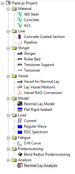
Project Sidebar for Example 15
When a new PipeLay project is created it contains just a Project component. This component is used to store general project information such as the project title, location, and so on. The Project component is also used to specify certain project-specific settings such as the system of units to be used, global constants, finite element mesh settings and quality control procedures. For this example, the following information is stored in the general Project Settings dialog.
Table: General Project Settings
Property |
Value |
Project Title |
Example 15 - Shallow Water Rigid S-Lay |
Job Number |
1-2-3-342 |
Engineer(s) |
Wood PLC |
Location |
Galway |
For this example, the default Metric unit system option is used, along with the default Quality Control selections. Under the Constants dialog however, the Maximum Element Length is specified as 2m (instead of 10m default) with the remaining entries selected as per default. This change in element length is a reflection of the shallow water nature of the scenario under consideration.
The Material component is used to define the physical properties associated with a particular material. This example contains three Material components: ‘X65 Steel’, ‘Concrete’ and ‘ACL’ (anti-corrosion layer). These are nonlinear materials specified by stress-strain curves, describing both tensile and compressive properties.
Table: Material Properties for ‘X65 Steel’
|
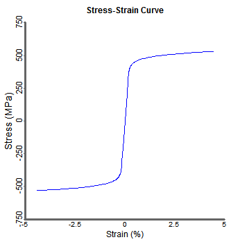 Stress-Strain Curve for ‘X65 Steel’ |
Table: Material Properties for ‘Concrete’
|
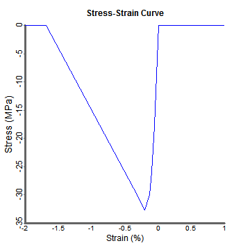 Stress-Strain Curve for ‘Concrete’ |
Table: Material Properties for ‘ACL’
|
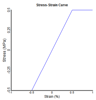 Stress-Strain Curve for ‘ACL’ |
The Pipe Section component is used to specify the properties of an individual section of pipeline that has uniform properties. This example contains one Pipe Section component as follows:
▪The Pipe Section component is created in the Line folder and is named ‘Concrete Coated Pipe’.
▪The specification is Standard.
▪The material used is ‘X65 Steel’’, as defined previously.
▪The geometrical and hydrodynamic properties are listed in the table below.
Table: Properties for ‘Concrete Coated Pipe’
Property |
Value |
Outer Diameter |
914.4 mm |
Thickness |
23.9 mm |
Normal Drag |
0.7 |
Normal Inertia |
2 |
The ‘X65 Steel’ pipe is applied two external coatings: an anti-corrosion coating and a concrete coating. Their properties are specified in the two tables below, respectively.
Table: Properties for ‘Anti-Corrosion Coating’
|
Table: Properties for ‘Concrete Coating’
|
The Line component is created in the Line folder and is named ‘Pipeline’. This Line component contains 500 m of the Pipe Section component ‘Concrete Coated Section’.
This example contains two Support components to model the supports on both the vessel and the stinger. Both Support components are created in the Stinger folder. One component is a Double V Support, named ‘Roller Bed’, and the other component is a Zero-Gap O Support, named ‘Tensioner Support’. The ‘Tensioner Support’ component has a support length of 4.9 m. The properties of the ‘Roller Bed’ component are listed in the table below.
Table: Properties of ‘Roller Bed’
Property |
Value |
Support Length |
2.45 m |
Roller Length, L1 |
0 m |
Roller Length, L2 |
1 m |
Roller Length, L3 |
1 m |
Roller Angle, Theta 1 |
30° |
Roller Angle, Theta 2 |
90° |
Contact Stiffness |
5000 kN/m |
Tensioner Component
A single Tensioner component is created in the Stinger folder and is named ‘Tensioner’. The Type is specified as Linear, while the Coefficient Type is specified as Active with default Damper properties. ‘Tensioner Support’, as its name suggests, is used as the Tensioner Support.
A Stinger component is used to model the rigid S-Lay stinger. This component is created in the Stinger folder and is named ‘Stinger’. Explicitly Defined is selected as the stinger definition option. The Support Locations on the stinger are listed in the table below. The coordinates provided here represent the initial support positions before any optimisation is applied.
Table: Support Locations on ‘Stinger’
Support Name |
X Coordinate (m) |
Y Coordinate (m) |
Roller Bed |
-0.22 |
-4.49 |
Roller Bed |
-2.2 |
-14.9 |
Roller Bed |
-4.63 |
-25.22 |
Roller Bed |
-7.51 |
-35.42 |
Roller Bed |
-10.84 |
-45.48 |
Roller Bed |
-14.61 |
-55.39 |
Roller Bed |
-18.82 |
-65.12 |
Roller Bed |
-23.45 |
-74.65 |
Roller Bed |
-28.5 |
-83.98 |
A Vessel component named ‘Vessel for Normal Lay’ is created in the Vessel folder. This component models the lay vessel. The Standard Vessel Profile option is selected from the Profile Options drop-down list. The overall dimensions of the vessel are listed in the table below.
Table: Properties of ‘Vessel for Normal Lay’
Property |
Value |
Length |
151.2 m |
Depth of Keel below Origin |
6.5 m |
Horizontal Offset from Origin |
75.6 m |
Create Solid Profile |
No |
The Vessel Reference Point, Stinger Location and Support Locations are all also defined in the Vessel component, the properties of which are listed in three tables below respectively.
Table: Reference Point of ‘Vessel for Normal Lay’
|
Table: Location of ‘Stinger’
|
Table: Support Locations on ‘Vessel for Normal Lay’
|
Radii of Curvature for the supports along the vessel and stinger are to be user-defined also. However, as mentioned in the Introduction section, this process is to be carried out over a number of iteration steps and each of these steps is described later in the Running the Analysis section of the Analysis Component.
To complete the specification of the Vessel component, the Vessel Motion component ‘Lay Vessel Motions’ is associated with the vessel by selecting it from the Vessel Motions drop-down list.
The Vessel Motion component is used to specify the dynamic motions of a vessel, including first order (RAO) motions and second order (drift) motions. This example contains a Vessel Motion component named ‘Lay Vessel Motions’ which is created in the Vessel folder. The vessel motion option RAO + Drift is selected from the Motion Type drop-down list. The RAO file included in the example directory, Lay Vessel.rao, is loaded into the component through the RAO File dialog. These RAOs are supplied in the Custom format meaning that a RAO Conversion component is required to convert the selected RAO data to the MCS Kenny format which is used by PipeLay. The RAO Conversion component ‘Vessel RAO Conversion’ is associated with the vessel by selecting it from the RAO Conversion drop-down list.
To view the RAO data, you can generate a PipeLay RAO Report by selecting Yes on the Plot RAOs drop-down list and then click on the Plot RAOs Button in the Vessel Motion Section of the Ribbon. This RAO Report contains graphs of the RAO and phase angles for each of the translational and rotational DOFs for the vessel. The Heave RAO plot is included in the figure below as an example.
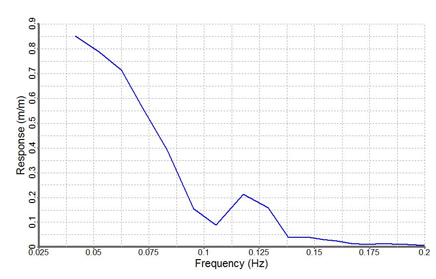
Heave RAOs for Lay Vessel
The RAO Conversion component is used to specify the method in which a selected Custom format RAO data file is converted to the MCS Kenny format which is then used by PipeLay. The RAO Conversion component is located in the Vessel folder. The RAO Conversion method created can be then selected from the drop-down list in the Vessel Motion component for use. The component is predominately made up of drop-down lists, the majority of which remain at their default selections for this example. The default selections correspond to the standard MCS Kenny RAO file format.
Selections that vary from the default are detailed in the table below as follows.
Table: Properties of ‘Vessel RAO Conversion’
Property |
Value |
Incident On… |
Stern |
Wave Units |
Frequency [rads/sec] |
+ve surge direction |
Aft |
+ve sway direction |
Starboard |
A single Seabed component is created in the Model folder and is named ‘Flat Rigid Seabed’. The default properties of a rigid seabed, with a zero coefficient of friction in the longitudinal and transverse directions and a slope of zero degrees, are left unchanged.
One Current component is created in the Load folder. The name of the component is ‘Current’ and is specified as Piecewise linear from the Type drop-down list and MWL in the Water Surface drop-down list. The Current Data is specified in the table below.
Table: Current Data for ‘Current’
Distance Below Mean Waterline [m] |
Velocity [m/s] |
0 |
0.41 |
10 |
0.41 |
69 |
0.16 |
Two Wave components are created in the Load folder. A component, named ‘Regular Wave’, is added to model the regular wave included in this example. The Regular option is selected from the Type drop-down list and the properties of the component are listed in the table below.
Table: Properties of ‘Regular Wave’
Property |
Value |
Amplitude |
1.5 m |
Period |
10 s |
Direction |
180° |
Phase |
0.0° |
A second Wave component, named ‘ISSC Spectrum’ is added to model the random sea included in the example. The User Specified – Equal Area Discretisation option is selected from the Type drop-down list and the Wave Data properties of the component are listed in the table below. The User Spectrum data for the ‘ISSC Spectrum’ is listed in the table below.
Table: Properties of ‘ISSC Spectrum’
Property |
Value |
Number of Harmonics |
100 |
Dominant Direction |
180° |
Table: User Spectrum data for ‘ISSC Spectrum’
Frequency [Hz] |
Spectral Value [m2.s] |
0.04 |
0.000013 |
0.042 |
0.000225 |
0.044 |
0.001995 |
0.046 |
0.010936 |
0.048 |
0.041548 |
0.05 |
0.118982 |
0.052 |
0.27347 |
0.054 |
0.528887 |
0.056 |
0.892221 |
0.058 |
1.349785 |
0.06 |
1.870996 |
0.062 |
2.416596 |
0.064 |
2.947279 |
0.066 |
3.430078 |
0.068 |
3.841625 |
0.07 |
4.168719 |
0.072 |
4.407114 |
0.074 |
4.559456 |
0.076 |
4.63307 |
0.078 |
4.637978 |
0.08 |
4.585343 |
0.082 |
4.486349 |
0.084 |
4.351481 |
0.086 |
4.190115 |
0.088 |
4.010337 |
0.09 |
3.818917 |
0.092 |
3.621373 |
0.094 |
3.422097 |
0.096 |
3.224495 |
0.098 |
3.03114 |
0.1 |
2.843914 |
0.102 |
2.66413 |
0.104 |
2.492654 |
0.106 |
2.329994 |
0.108 |
2.176383 |
0.11 |
2.031843 |
0.112 |
1.896243 |
0.114 |
1.769336 |
0.116 |
1.650797 |
0.118 |
1.540248 |
0.12 |
1.43728 |
0.122 |
1.341466 |
0.124 |
1.252377 |
0.126 |
1.169585 |
0.128 |
1.092675 |
0.13 |
1.021246 |
0.132 |
0.954916 |
0.134 |
0.893321 |
0.136 |
0.836118 |
0.138 |
0.782986 |
0.14 |
0.733625 |
0.142 |
0.687753 |
0.144 |
0.645111 |
0.146 |
0.605456 |
0.148 |
0.568564 |
0.15 |
0.534227 |
0.152 |
0.502255 |
0.154 |
0.472469 |
0.156 |
0.444706 |
0.158 |
0.418816 |
0.16 |
0.394659 |
0.162 |
0.372108 |
0.164 |
0.351044 |
0.166 |
0.331359 |
0.168 |
0.312951 |
0.17 |
0.295729 |
0.172 |
0.279607 |
0.174 |
0.264507 |
0.176 |
0.250355 |
0.178 |
0.237086 |
0.18 |
0.224636 |
0.182 |
0.21295 |
0.184 |
0.201974 |
0.186 |
0.191659 |
0.188 |
0.181961 |
0.19 |
0.172837 |
0.192 |
0.164249 |
0.194 |
0.156162 |
0.196 |
0.148542 |
0.198 |
0.141358 |
0.2 |
0.134583 |
0.202 |
0.12819 |
0.204 |
0.122153 |
0.206 |
0.116451 |
0.208 |
0.111063 |
0.21 |
0.105968 |
0.212 |
0.101148 |
0.214 |
0.096587 |
0.216 |
0.092269 |
0.218 |
0.088178 |
0.22 |
0.084302 |
0.222 |
0.080626 |
0.224 |
0.07714 |
0.226 |
0.073832 |
0.228 |
0.070692 |
0.23 |
0.067709 |
0.232 |
0.064875 |
0.234 |
0.062182 |
0.236 |
0.059621 |
0.238 |
0.057185 |
0.24 |
0.054866 |
0.242 |
0.052659 |
0.244 |
0.050557 |
0.246 |
0.048555 |
0.248 |
0.046646 |
0.25 |
0.044826 |
An S-N Curve component named ‘S-N Curve’ is created in the Fatigue folder. This component is used during the fatigue analysis. The Curve Type is specified as Linear and the Properties specifying the curve are listed in the table below.
Table: ‘S-N Curve’ Properties
Property |
Value |
m |
3.0 |
K |
1.1192 x 10¹² (MPa)m |
Endurance Limit |
0.0 MPa |