<< Click to Display Table of Contents >> Navigation:  PipeLay > Example PipeLay Models > Example 13 - Pipe-in-Pipe >
Components

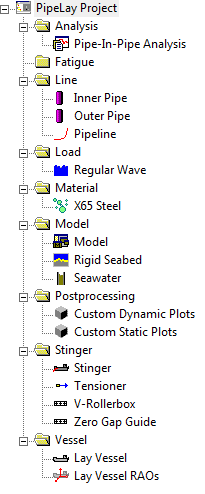
The project sidebar for this example is shown in the figure below. The project sidebar shows all of the components that are used in the example. Each of these components is described in detail in the following sections.

 

 

Project Component

When a new PipeLay project is created it contains just a Project component. This component is used to store general project information such as the project title, location, and so on. The Project component is also used to specify certain project-specific settings such as the system of units to be used, global constants, finite element mesh settings and quality control procedures. For this example, the following information is stored in the general Project Settings dialog.

Table: General Project Settings

In the case of this example, many of the default project-specific settings are used (e.g. metric unit system, default water density etc.). However, in order to accurately model the interaction between the outer and inner pipes, the Maximum Element Length is reduced to 2m.

Back to Overview

 

Material Component

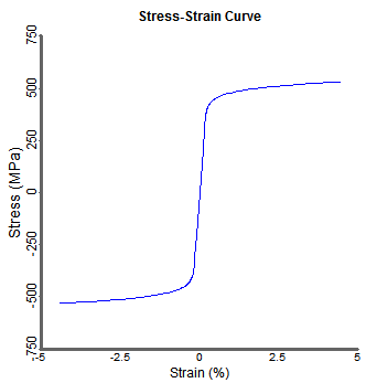
The Material component is used to define the physical properties associated with a particular material. This example contains one Material component, which defines the nonlinear material properties for X65 steel, as listed in the table below. The Material component is created in the Material folder and is named ‘X65 Steel’ in this example.

Table: Material Properties for ‘X65 Steel’

 

 

Pipe Section Component

The Pipe Section component is used to specify the properties of an individual section of pipeline that has uniform properties. There are two pipe sections used in this project, for outer and inner pipes as follows:

▪The Pipe Section components are located in the Line folder and is named ‘Outer Pipe’ and ‘Inner Pipe’, respectively.

▪The specification in both cases is Standard.

▪The material used in both cases is ‘X65 Steel’, as defined previously.

▪The geometrical and hydrodynamic properties are listed in the table below.

Table: Summary of Pipe Section Properties

Back to Overview

 

Line Component

The Line component is created in the Line folder and is named ‘Pipeline’, contains 1050m of the Pipe Section component ‘Outer Pipe’. The pipe-in-pipe properties are also specified on the Line component, by selecting the Pipe In Pipe tab and the Define Inner Section button. These properties are given in the table below. The interaction between the outer pipe and the inner pipe, at locations where no bulkheads or centralisers are present, is modelled using the default force-displacement curve provided by PipeLay. Bulkheads are located at the start and end of the line, and the two pipes are connected together at these points by sharing common nodes. The centralisers fill the entire gap between the outer and inner pipes.

Table: Pipe-In-Pipe Properties

 

Support Components

This example contains two Support components to model the supports on both the vessel and the stinger. Both Support components are created in the Stinger folder. One component is a Double V Support, named ‘V-Rollerbox’, and the other component is a Zero Gap O Support, named ‘Zero Gap Guide’. The ‘Zero Gap Guide’ component has a support length of 5 m. The properties of the ‘V-Rollerbox’ component are listed in the table below.

Table: Properties of ‘V-Rollerbox’

Back to Overview

 

Tensioner Component

A single Tensioner component is created in the Stinger folder and is named ‘Tensioner’. The Type is specified as Linear, while the Coefficient Type is specified as Active with default Damper properties. ‘Zero-Gap Guide’ is used as the Tensioner Support.

 

Stinger Component

A Stinger component is created to model the S-Lay stinger. This component is created in the Stinger folder and is named ‘Stinger’. Radius of Curvature Defined is selected as the stinger definition option. The Support Locations on the stinger are listed in the table below.

Table: Support Locations on ‘Stinger’

 

The Support Locations correspond to the curvilinear distance along the arc from the top of the stinger, which is defined as being directly below the Centre of Curvature. The Centre of Curvature for the stinger is defined in the table below.

Table: Centre of Curvature for ‘Stinger’

Back to Overview

 

Vessel Component

A Vessel component named ‘Lay Vessel’ is created in the Vessel folder. This component models the lay vessel. The Standard Vessel Profile option is selected from the Profile Options drop-down list. The overall dimensions of the vessel are listed in the table below.

Table: Properties of ‘Lay Vessel’

 

The Vessel Reference Point, Stinger Location and Support Locations are all also defined in the Vessel component, the properties of which are listed in the three tables below respectively.

Table: Reference Point of ‘Lay Vessel’

 

Table: ‘Stinger’ Location

 

Table: Support Locations on ‘Lay Vessel’

 

To complete the definition of the Vessel component, the Vessel Motion component ‘Lay Vessel RAOs’ is associated with the vessel by selecting it from the Vessel Motions drop-down list.

Back to Overview

 

Vessel Motion Component

The Vessel Motion component is used to specify the dynamic motions of a vessel, including first order (RAO) motions and second order (drift) motions. This example contains a Vessel Motion component named ‘Lay Vessel RAOs’, which is created in the Vessel folder. The vessel motion option RAO + Drift is selected from the Motion Type drop-down list. The RAO file included in the example directory, Lay Vessel.rao, is loaded into the component through the RAO File dialog. These RAOs are supplied in the MCS Kenny format, so the remaining options are left unchanged.

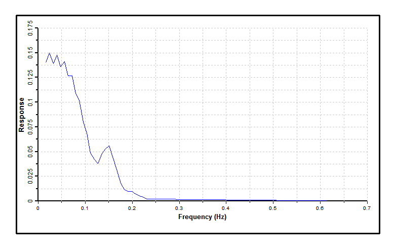
To view the RAO data, you can generate a PipeLay RAO Report by selecting Yes on the Plot RAOs drop-down list. This RAO Report contains graphs of the RAO and phase angles for each of the translational and rotational DOFs for the vessel. The Heave RAO plot is included in the figure below as an example.

 

Seabed Component

A single Seabed component is created in the Model folder and is named ‘Rigid Seabed’. The default properties of a rigid seabed, with a zero coefficient of friction in the longitudinal and transverse directions and a slope of zero degrees, are left unchanged.

 

Internal Fluid Component

The Internal Fluid component is used to specify the properties of an internal fluid for a pipeline. In this example, an Internal Fluid component named ‘Seawater’ is created in the ‘Model’ folder to model the flooding of the pipeline. Naturally it has a mass density of 1025kg/m3.

 

Wave Component

A single Wave components is added to the Load folder, named ‘Regular Wave’. This Wave component is used to model the regular wave included in this example. The Regular option is selected from the Type drop-down list and the properties given in the table below.

Table: Properties of ‘Regular Wave’

Back to Overview