<< Click to Display Table of Contents >> Navigation:  PipeLay > Example PipeLay Models > Example 02 - Normal J-Lay >
Components

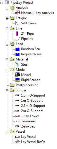
The project sidebar for this example is shown in the figure below. The project sidebar shows all of the components that are used in the example. Each of these components is described in detail in the following sections.

 

Project Component

When a new PipeLay project is created it contains just a Project component. This component is used to store general project information such as the project title, location, and so on. The Project component is also used to specify certain project-specific settings such as the system of units to be used, global constants, finite element mesh settings and quality control procedures. For this example, the following information is stored in the general Project Settings dialog.

Table: General Project Settings

For this example, the default Metric unit system and the default Constants dialog values are used. Also, the ‘Quality Control’ section is left as per default.

Back to Overview

Material Component

The Material component is used to define the physical properties associated with a particular material. This example contains one component, which defines the material properties for steel, as listed in the table below. The Material component is located in the Material folder and is named ‘Steel’ in this example.

Table: Material Properties for ‘Steel’

 

Pipe Section Component

The Pipe Section component is used to specify the properties of an individual section of pipeline that has uniform properties. This example contains one Pipe Section component as follows:

▪The Pipe Section component is created in the Line folder and is named ‘24’’ Pipe’.

▪The specification is Standard.

▪The material used is ‘Steel’, as defined previously.

▪The geometrical and hydrodynamic properties are listed in the table below.

Table: Properties for ‘24’’ Pipe’

Back to Overview

Line Component

The Line component is created in the Line folder and is named ‘Pipeline’. This Line component contains 2000m of the Pipe Section component ‘24’’ Pipe’.

 

Support Components

Support components are created to model the rollerboxes on the J-Lay tower. This example contains five support types, created in the Stinger folder. The support names, types, and specifications are listed in the table below. The support types are selected from the Support Type drop-down list and the specifications are entered in the Support Properties dialog.

Table: Properties of Support Components

 

 

Tensioner Component

A Tensioner component named ‘Tensioner’ is created in the Stinger folder. This component models the tensioner at the top of the tower. The Type is specified as Linear, while the Coefficient Type is specified as Active with default Damper properties. ‘Zero Gap’ is used as the Tensioner Support.  

 

Stinger Component

A Stinger component named ‘J-Lay Tower’ is created in the Stinger folder. This component models the J-Lay Tower. J-Lay is selected as the stinger Type and the Support Locations listed in the table below are specified. A Tower Angle of -80° is specified in the Tower Properties dialog.

Table: Support Locations on ‘J-Lay Tower’

Back to Overview

Vessel Component

A Vessel component named ‘Lay Vessel’ is created in the Vessel folder. This component models the lay vessel. User Vessel Profile is selected from Profile Options and the profile in the file Lay Vessel.ves is loaded through the User Specified Profile dialog. The default zero translational offsets are used. The previously defined tower is then associated with the vessel by selecting the Tower component ‘J-Lay Tower’ from the Stinger drop-down list. The stinger reference point is left unchanged from the default values in the Location dialog. The Vessel Motion component is associated with the vessel by selecting Lay Vessel RAOs from the Vessel Motions drop-down list.

 

Vessel Motion Component

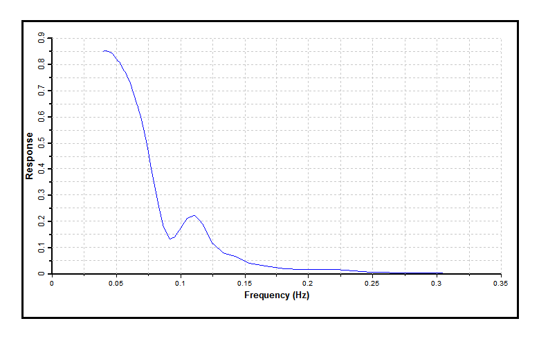
A Vessel Motion component named ‘Lay Vessel RAOs’ is created in the Vessel folder. This component is used to specify the dynamic responses of the lay vessel. The vessel Motion Type is selected as RAO + Drift and the RAO file for the project, Lay Vessel.rao, is loaded through the RAO File dialog. The RAOs are supplied in MCS Kenny format, so no RAO format conversion is required. The Heave RAO plot is included in the figure below as an example.

Seabed Component

A Seabed component named ‘Rigid Seabed’ is created in the Model folder. The default seabed properties of a rigid seabed, with a zero coefficient of friction in the longitudinal and transverse directions and a slope of zero degrees, are left unchanged.

Back to Overview

Wave Component

Two Wave components named ‘Regular Wave’ and ‘Random Sea’ are created in the Load folder. These components are used to define the wave loadings present in the example. ‘Regular Wave’ is added to model the regular wave included in the example. The Regular option is selected from the Type drop-down list. The regular wave has an amplitude of 4.0m and a period of 8s, in a direction of 180°. A second Wave component, ‘Random Sea’, is added to model the random sea included in the example. The Pierson-Moskowitz – Equal Area Discretisation option is selected from the Type drop-down list and the properties listed in the table below are entered.

Table: Properties of ‘Random Sea’

 

S-N Curve Component

An S-N Curve component named ‘S-N Curve’ is created in the Fatigue folder. This component is used during the fatigue analysis. The Curve Type is specified as Linear and the coefficients specifying the curve that are listed in the table below are entered in the Properties dialog.

Table: ‘S-N Curve’ Properties

Back to Overview